How to Use Excel to Track Vacation Schedules

Supervisors, are you setting up your vacation schedule?

With so many people to manage, and so many vacation requests, how can you use Excel to track all your employees and their requests?

Method 1: (Not best)

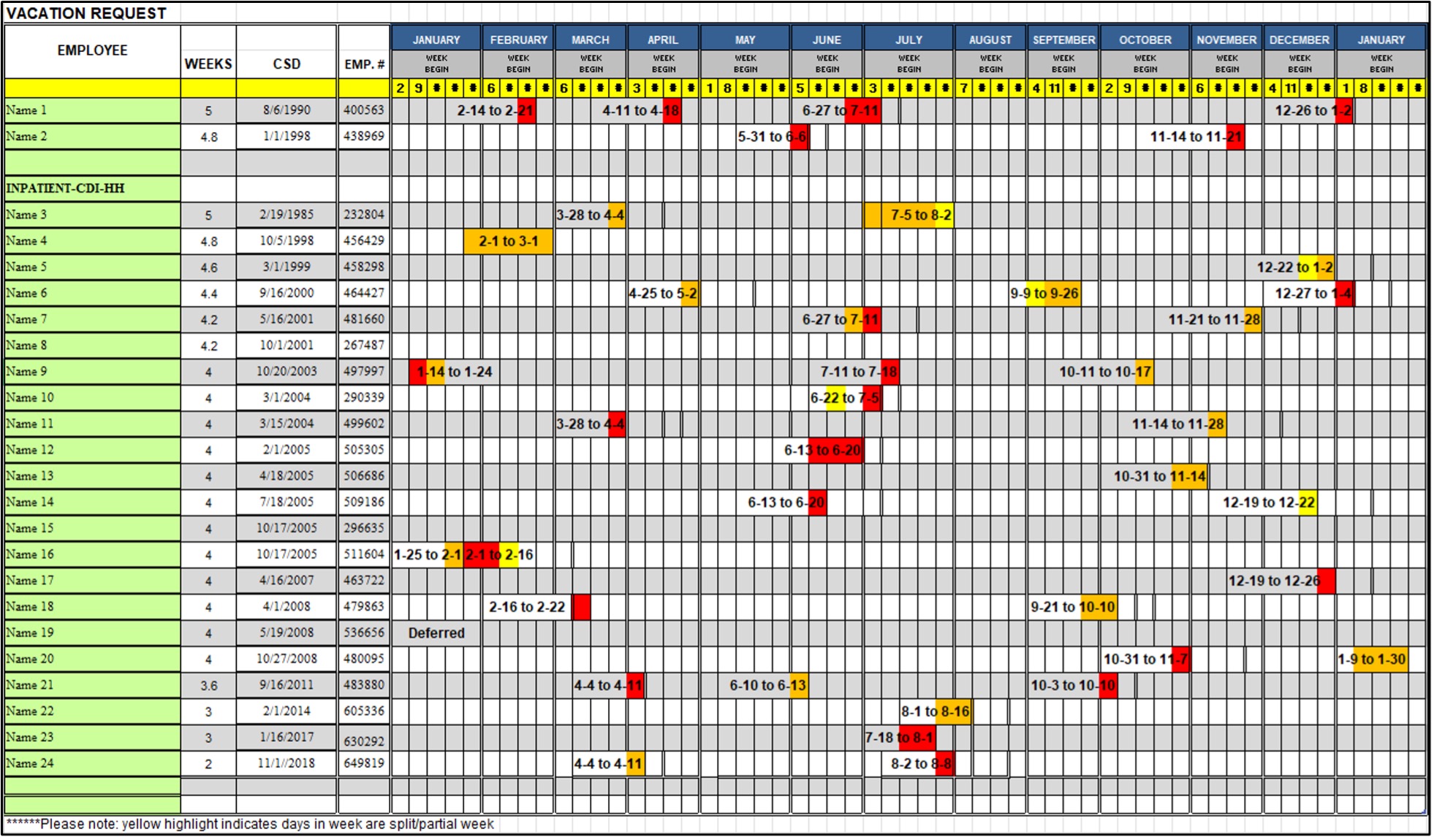
You could create a big “visual” and manually color coat each day of the year. However, it’s too big to print on a single piece of paper.

Method 2: (Better)

Put on your thinking cap and

1. Do what you’ve learned in Excel training: Make a Table, and
2. Figure out how to “work around” a formula “problem.”

Using Excel’s Tables to Track Vacation

The heart and soul of data management in Excel is the Table. Create a column of Vacation Dates and a Column for Requester.

The right Excel formula to help track vacation

This is where there’s a problem! If you write a classic “COUNTIF” formula, the formula will fail to respect any filters you apply to the list.

For example, you might only allow a certain number of employees to be on vacation at a time — but Supervisors are exempt from that restriction!

So, when you filter out supervisors, the COUNTIF column does not “subtract” their vacation days from the total people off on any given date!

Not good!

You don’t want your beautiful table and calculation to be accompanied by an “excuse” like “It kind of works… but not exactly.”

So, you need to write a formula in another column that only counts the rows that are displayed, and doesn’t count hidden rows.

In a way, you could say,

1. Is it counted?
2. Is it visible?

If these two statements are both TRUE, you COUNT the day off.

How do you do this? With SUMPRODUCT and SUBTOTAL because SUMPRODUCT counts people who are on vacation and SUMPRODUCT counts only visible rows.

If a row is a day off, and is visible, COUNT IT!

In general terms, your formula looks like:

Looked at another way, you could say:

The Result of both sides of the SUMPRODUCT function would look like:

Which would be calculated as:

With this formula, the result would be 1 (Only a total of 1 Person asked for a day off) . ((1 * 1) + (0 * 1) + (0 * 0). In other words, 1.

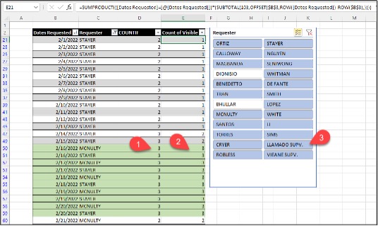
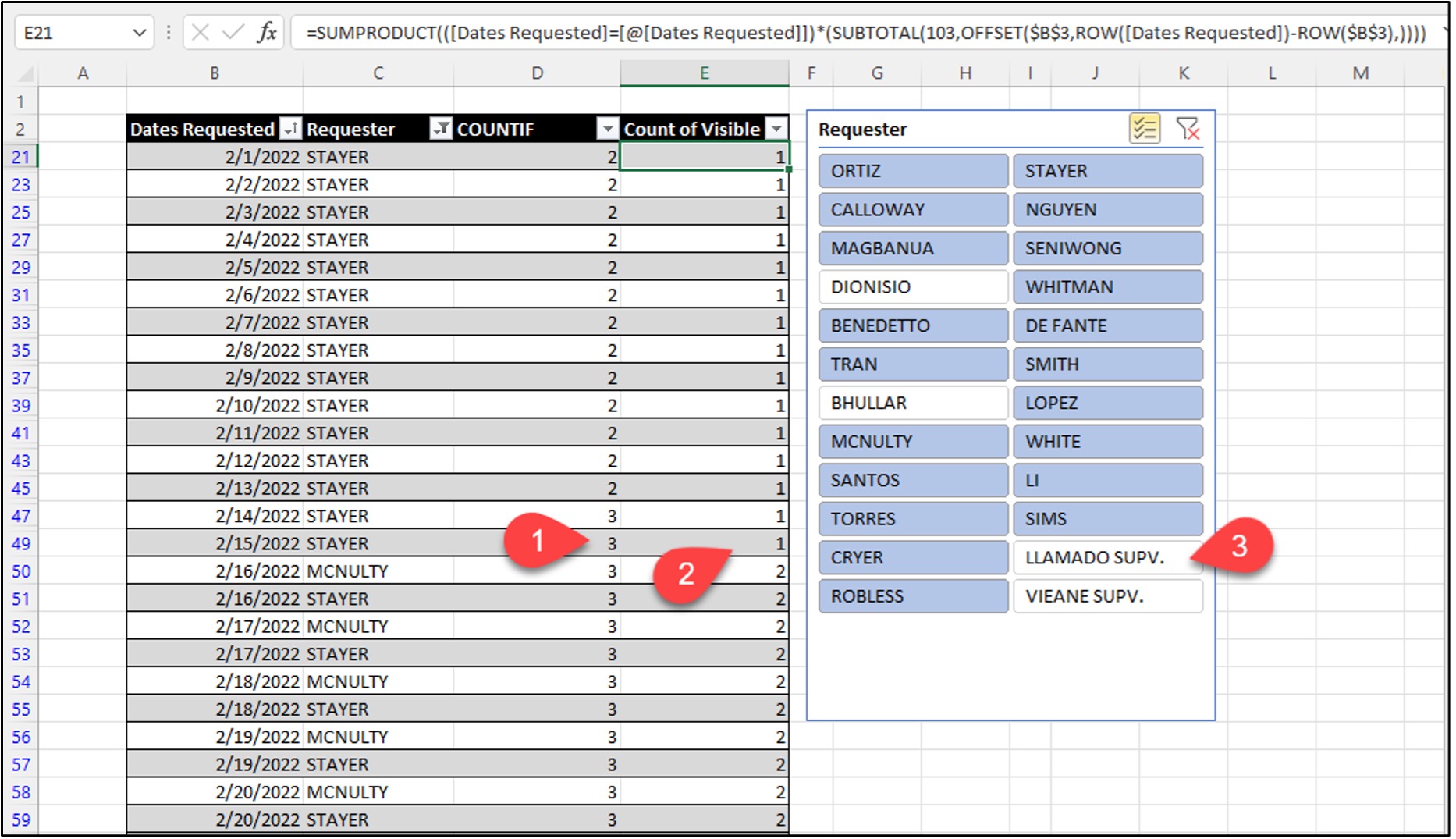
In this example, we have some folks who have chosen vacation dates that amount to 3 off at one time! CF (Conditional Formatting) of the table highlights this.

But, once we filter out the supervisors (Llamado and Vieane) we are no longer “over the limit.”

When you compare the two formulas, COUNTIF and Count of Visible, you see how the COUNTIF column continues to COUNT all rows (visible or hidden) while the SUMPRODUCT-driven calculation (Count of Visible) only includes the count of visible rows.

Breaking it down further:

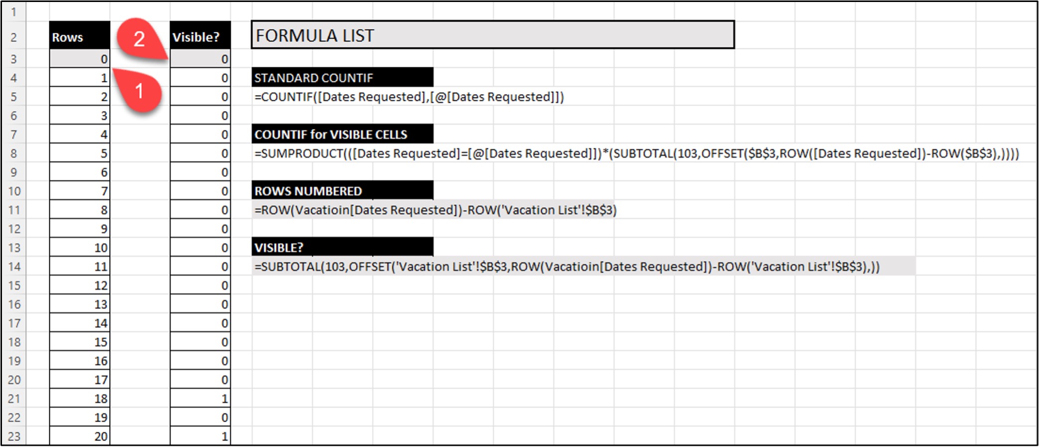
The failed formula is a simple COUNTIF formula:

In comparison, the complete COUNT OF VISIBLE FORMULA is:

Let’s break it down!

We know the first half of the SUMPRPODUCT formula, finds the rows with date matches:

The second half of the SUMPRODUCT formula finds which rows are “not hidden”:

The argument, 103 means “COUNT and (this is important!) Ignore Hidden Rows.

• The argument, ROW([Dates Requested])-ROW($B$3),))) returns a list of rows from 0 to the last row number in the array.
• The joint functions, SUBTOTAL and OFFSET count whether each returned row is visible.

In the illustration below, notice the column titled “Visible” has 0’s and 1’s. (0 means it is hidden, 1 means it is visible).

Finally, when you pack all three functions, SUMPRODUCT, SUBTOTAL, and OFFSET together — you get what you need — an easy way to COUNT the number of people on vacation — with or without filtering out supervisors!

The Excel Insider’s Club

When you highlinght the first “section” of the formula and press the F9 function key, you can see the “inside” calculation for “criteria”.

When you highlight the second “section” of the formula and press the F9 function key, you can see the “insider” calculation for “visibility.”

---

Ready to learn more? Check out some of SkillPath’s live virtual training programs, on-demand video training or get it all with our unlimited eLearning platform.